Linear models are powerful, but also have important restrictions:
straight line relationships at some point become negative, which may not be realistic
for inference, variation around the regression surface has to be normally distributed
Transforming the dependent variable non-linearly (e.g. taking a logarithm, or do some Box-Cox transformation), but these not always solve all problems and may create new ones.
Generalized linear models extend (generalize) the linear model for certain common data types, in particular count data and binary data. The model is formulated as
\[g(E(y|X)) = X\beta \]
or alternatively
\[\mu(X) = E(y|X) = g^{-1}(X\beta)\]
The link function\(g(\cdot)\) guarantees that the mean function stays in the valid data range, meaning
for count data it will not remain positive (or not become negative), we typically use \(g(x) = \log(x)\)
for binomial data, it will remain inside the range \((0,1)\), we typically use the logit function \(g(x)=\log(x/(1-x))\)
A problem that arises is that observations cannot directly be transformed: for Poisson variables, zero counts lead to \(-\infty\), for binomial variables zero and one lead to \(-\infty\) and \(\infty\), so models cannot be fitted directly to the data.
NoteExercise
How is the parameter vector \(\beta\) estimated in generalized linear models?
NoteExercise
How does a first order linear model (\(y=a+bx+e\)) look like on the 0-1 (observation) scale? How is it called? How does a second-order linear model look like on the same scale?
A further complication in GLMs is that the variance is not constant, for instance
for Poisson variables, \(Var(y|x) = \mu(x)\)
for binomial variables, \(Var(y|x) = \mu(x)(1-\mu(x))\)
Weighted least squares is used to include these weights, but iteration is needed: for the weights we use the estimated mean (from the previous iteration) to update the parameter estimate (in the current iteration), until convergence.
In R, the glm() function fits GLMs. Its second argument, family, defines the combination of link function and variance function.
For count data, a very common case is overdispersion, which means that the variance of \(y\) is larger than \(\mu(x)\); we can use a negative binomial family for variables that have overdispersion, \(Var(y|x) = \phi \mu(x)\) with parameter \(\phi > 1\) fitted along with \(\beta\). For \(\phi=1\) it reduces to the Poisson family.
Note that neural networks are based on multiple, layered logistic regression models. We can think of logistic regression as a single-layer, single-output neural network with a sigmoid activation (a first-order linear effect).
Also note that linear models are a special case of generalized linear models, with an identity link function \(g(x)=x\) and a constant variance function \(Var(y|x)=\sigma^2\).
3.1 Covid-19 data from RKI
We downloaded Covid-19 counts per day per Landkreis from the Robert-Koch websites (up-to-date file found here; GitHub repo), and imported it in R, after zipping it:
Rows: 1009827 Columns: 7
── Column specification ────────────────────────────────────────────────────────
Delimiter: ","
chr  (1): Landkreis_id
dbl  (5): Bevoelkerung, Faelle_gesamt, Faelle_neu, Faelle_7-Tage, Inzidenz_7...
date (1): Meldedatum

ℹ Use `spec()` to retrieve the full column specification for this data.
ℹ Specify the column types or set `show_col_types = FALSE` to quiet this message.
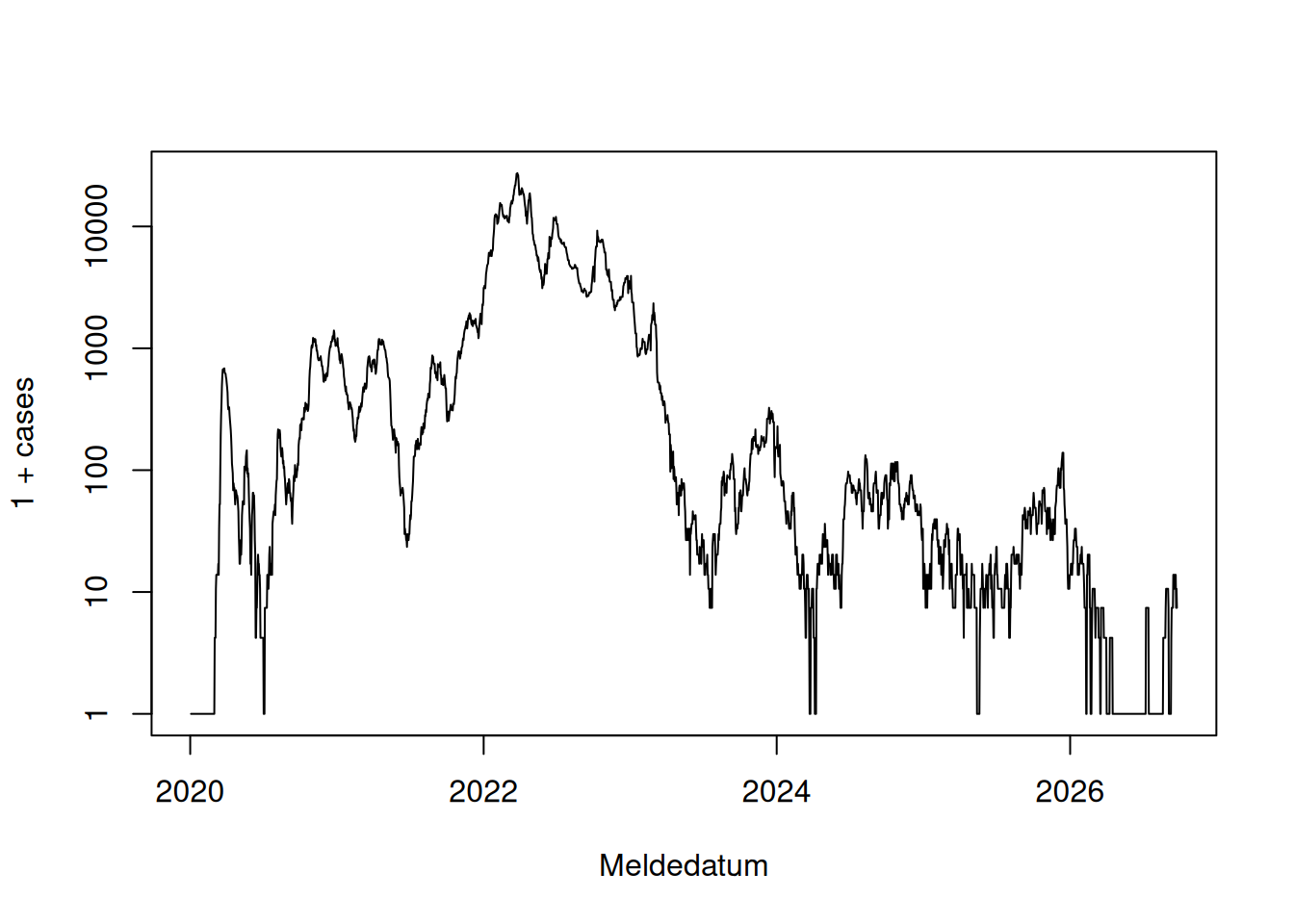
Then, we select Landkreis 5515 (Stadt Münster), and plot the variable cases, using a log-scale after adding 1:
Why do we specify the Date column class? Why do we plot using log-scale? Why plot this particular variable? Why do we add 1?
NoteExercise
Describe the curve thus obtained.
How can we describe the temporal pattern with regression models? The overall trend seems either linear (general decrease) or quadratic (increase followed by decrease), there may be seasonal effect (more cases in autumn/winter?)
We can first subsample the 7-day running means to weekly values without loosing much:
c19.MS.w = c19.MS |>mutate(d =as.numeric(Meldedatum), # day, as numberd_s =scale(d), # scaled to mean 0 sd 1d_rad =2* pi * d /365.25) |># day, yearday -> [0,2*pi]filter(d %%7==0)
NoteExercise
What exactly is lost by subsampling this way, compared to the 7-day running mean?
m =glm(round(cases)~d_s+I(d_s^2)+sin(d_rad)+cos(d_rad), c19.MS.w, family ="poisson")summary(m)
Call:
glm(formula = round(cases) ~ d_s + I(d_s^2) + sin(d_rad) + cos(d_rad),
    family = "poisson", data = c19.MS.w)

Coefficients:
             Estimate Std. Error z value Pr(>|z|)
(Intercept)  6.834342   0.004248 1608.88   <2e-16 ***
d_s         -7.293627   0.015204 -479.71   <2e-16 ***
I(d_s^2)    -6.900232   0.013639 -505.91   <2e-16 ***
sin(d_rad)   0.606128   0.002188  277.07   <2e-16 ***
cos(d_rad)   0.142904   0.002094   68.23   <2e-16 ***
---
Signif. codes:  0 '***' 0.001 '**' 0.01 '*' 0.05 '.' 0.1 ' ' 1

(Dispersion parameter for poisson family taken to be 1)

    Null deviance: 1513858  on 350  degrees of freedom
Residual deviance:  325007  on 346  degrees of freedom
AIC: 327218

Number of Fisher Scoring iterations: 7
# m = MASS::glm.nb(round(cases)~d_s+I(d_s^2)+sin(d_rad)+cos(d_rad), c19.MS.w, start = c(1,rep(0,4)))# summary(m)
NoteExercise
Interpret the output, and compare it with a model that has only a first order linear effect. What is meant by deviance?
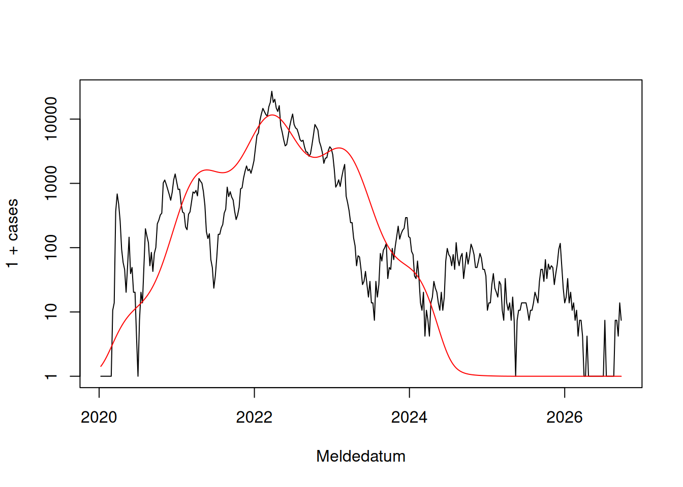
We can see how (well) this model predicts over the observed period:
plot(1+cases ~ Meldedatum,c19.MS.w, type ='l', log ="y")lines(c19.MS.w$Meldedatum, 1+exp(predict(m)), col ='red')
NoteExercise
What is good in the fit, and what is not so good? What may be a cause of a bad fit?
NoteExercise
Reflect on the assumptions made for this regression, in particular the one of independence of residuals.