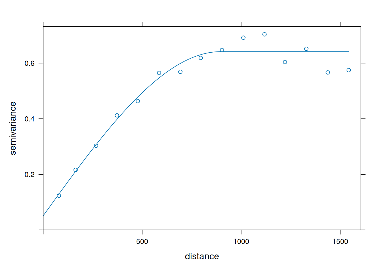
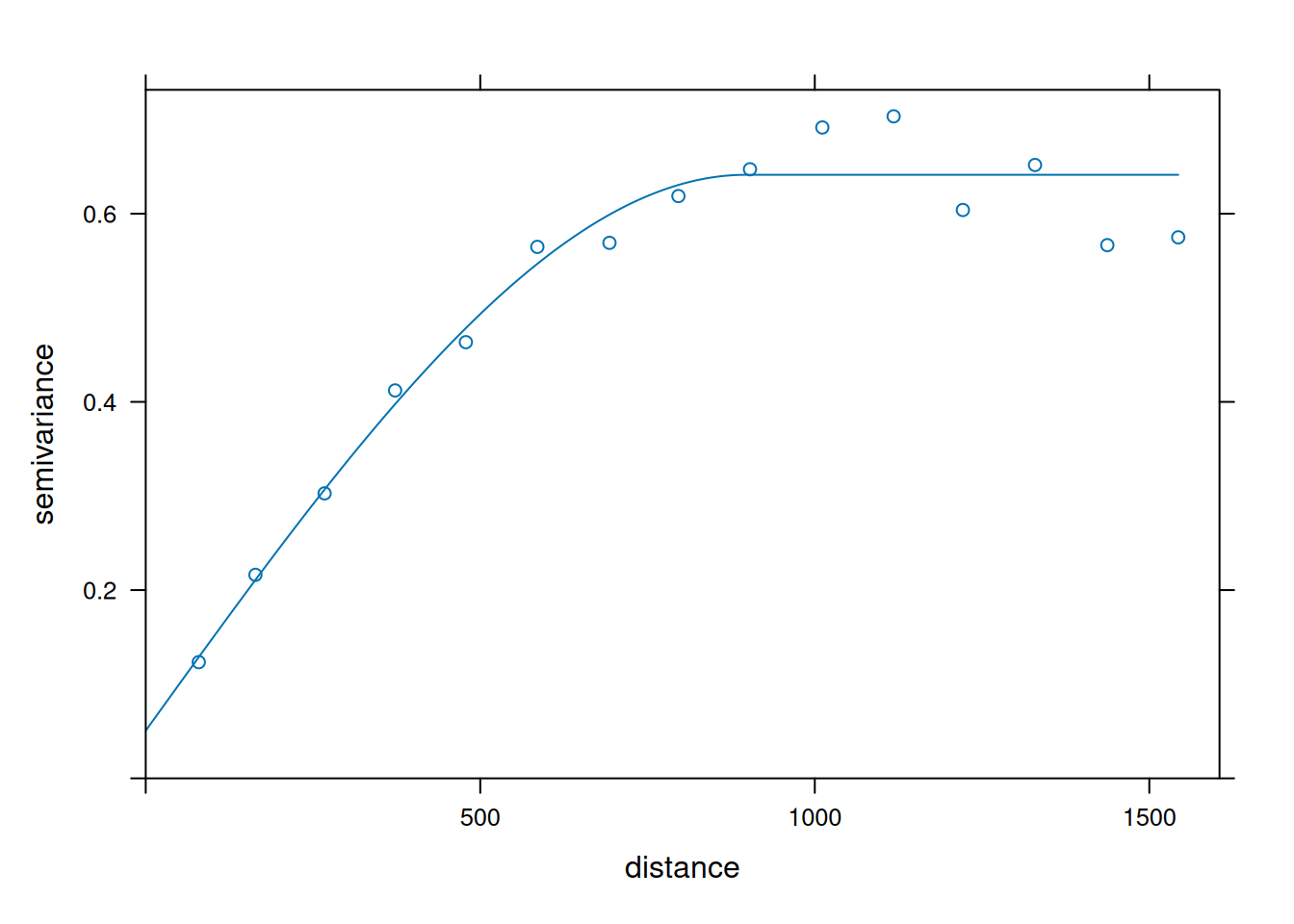
We can think of a Gaussian process as a collection of random variables that follow a multivariate Gaussian distribution, as in \[y(s) = \beta_0 + e(s), e(s) \sim \mathcal{N}(0,\Sigma)\] with \(\Sigma_{ij}=Cov(e(s_i),e(s_j))\) (which is a variance if \(i=j\)). The index \(s\) indicates that \(y(s)\) might be a spatial, temporal, or spatiotemporal process. \(\beta_0\) can be estimated by generalized least squares, but the interest usually lies in predicting (estimating) \(y(s_0)\) at an unobserved location \(s_0\) from \(n\) observed values \(y(s_i), i = 1,...,n\). Given known \(\beta_0\) and \(\Sigma\), and with \(\Sigma_0\) the covariance between scalar \(y(s_0)\) and vector \(y(s)\), we get \[\hat{y}(s_0)=\beta_0 + \Sigma_0 \Sigma^{-1}(y(s)-\beta_0)\] which reduces to \(\beta_0\) when \(y(s_0)\) is uncorrelated with the other \(y(s)\) (and \(\Sigma_0\) is a vector with zeroes). This predictor is the best linear predictor, Gaussian process regression, and in spatial context also known as simple kriging.
In more realistic situations, \(\beta_0\) is not known (ordinary kriging) or a linear model \(X(s)\beta\) with unknown parameter vector \(\beta\) is assumed for the mean function (universal kriging). In that case, the generalized least squares (GLS) estimate for \(\beta=(X'\Sigma^{-1}X)^{-1}X'\Sigma^{-1}y(s)\) is substituted, giving \[\hat{y}(s_0)=x_0\hat{\beta}+\Sigma_0\Sigma^{-1}(y(s)-X\hat{\beta})\] with \(x_0\) the vector with predictor values corresponding to \(s_0\). In practice, when e.g. spatially predicting values over a regular grid covering the target region, for each \(s_0\) only \(x_0\) and \(\Sigma_0\) change, all other parts remain constant.
5.1 Spatial GP regression in practice
The theory of GP is pretty straightforward, the practice a bit harder:
one needs to come up with plausible covariance matrices \(\Sigma\) and \(\Sigma_0\), in particular one that is (always) invertible
inverting \(\Sigma\) may be cumbersome, if not prohibitive, if the number of observations is large (say, \(\gg 10^4\)); Heaton et al. (2019) explains and compares several approaches for making these models work for larger datasets
5.2 Spatial correlation from irregular data
\[
\newcommand{\E}{{\rm E}} % E expectation operator
\newcommand{\Var}{{\rm Var}} % Var variance operator
\newcommand{\Cov}{{\rm Cov}} % Cov covariance operator
\newcommand{\Cor}{{\rm Corr}}
\] ### Unknown, constant mean Suppose the mean is constant, but not known. This is the most simple realistic scenario. We can estimate it from the data, taking into account their covariance (i.e., using weighted averaging, or GLS):
\[\hat{\beta}_0 = ({\bf 1}'\Sigma^{-1}{\bf 1})^{-1} {\bf 1}'\Sigma^{-1}y(s)\] with \({\bf 1}\) a conforming vector with ones, and substitute this mean in the SK prediction equations: BLUP/Ordinary kriging: \[\hat{y}(s_0) = \hat{\beta}_0 + v'V^{-1} (y(s)-\hat{\beta}_0)\] Which has prediction error variance \[\sigma^2(s_0) = \sigma^2_0 - \Sigma_0'\Sigma^{-1}\Sigma_0 + Q\] with \(\sigma^2_0\) = var(y(s))$ and \(Q = (1 - {\bf 1}'\Sigma^{-1}\Sigma_0)'({\bf 1}'\Sigma^{-1}{\bf 1})^{-1}(1 - {\bf 1}'\Sigma^{-1}\Sigma_0)\)
5.2.1 Stationarity 1
Given prediction location \(s_0\), and data locations \(s_1\) and \(s_2\), we need: \(\Var(y(s_0))\), \(\Var(y(s_1))\), \(\Var(y(s_2))\), \(\Cov(y(s_0),y(s_1))\), \(\Cov(y(s_0),y(s_2))\), \(\Cov(y(s_1),y(s_2))\).
How to get these covariances?
given a single measurement \(y(s_1)\), we can not infer \(\Var(y(s_1))\)
given two measurements \(y(s_1)\) and \(y(s_2)\), we can never infer \(\Cov(y(s_1),y(s_2))\)
geven a time series at \(s_1\) and \(s_2\), we could estimate
\(C(h)\) needs (an estimate of) \(\beta_0\), \(\gamma(h)\) does not
\(C(0)\) may not exist (\(\infty\)!), when \(\gamma(h)\) does (e.g., Brownian motion: linear or power variogram)
5.3 Fitting covariance/semivariance models
5.4 Kriging
$$ % E expectation operator % Var variance operator % Cov covariance operator
For this, we need to know how the mean varies. Suppose we model this as a linear regression model in \(p\) known predictors: \[y(s_i) = \sum_{j=0}^p \beta_j X_j(s_i) + e(s_i)\]\[y(s) = \sum_{j=0}^p \beta_j X_j(s) + e(s) = X(s)\beta + e(s)\] with \(X(s)\) the matrix with predictors, and row \(i\) and column \(j\) containing \(X_j(s_i)\), and with \(\beta =
(\beta_0,...\beta_p)\). Usually, the first column of \(X\) contains zeroes in which case \(\beta_0\) is an intercept.
Predictor: \[\hat{y}(s_0) = x(s_0)\hat{\beta} + v'V^{-1} (y-X\hat{\beta}) \] with \(x(s_0) = (X_0(s_0),...,X_p(s_0))\) and \(\hat{\beta} = (X'V^{-1}X)^{-1} X'V^{-1}Z\) it has prediction error variance \[\sigma^2(s_0) = \sigma^2_0 - \Sigma_0'\Sigma^{-1}\Sigma_0 + Q\] with \(Q = (x(s_0) - X'\Sigma^{-1}Sigma_0)'(X'\Sigma^{-1}X)^{-1}(x(s_0) - X'\Sigma^{-1}\Sigma_0)\)
This form has several names: external drift kriging, universal kriging or regression kriging.
Example in meuse data set: log(zinc) depending on sqrt(meuse)
Plotting them:
5.4.1 With a linear trend in the coordinate
5.4.2 … and Gaussian covariance:
5.4.3 Estimating spatial correlation under the UK model
As opposed to the ordinary kriging model, the universal kriging model needs knowledge of the mean vector in order to estimate the semivariance (or covariance) from the residual vector: \[\hat{e}(s) = y(s) - X\hat\beta\] but how to get \(\hat\beta\) without knowing \(V\)? This is a chicken-egg problem. The simplest, but not best, solution is to plug \(\hat{\beta}_{OLS}\) in, and from the \(e_{OLS}(s)\), estimate \(V\) (i.e., the variogram of \(y(s)\))
OK: fill in a column vector with ones for \(X\): \(X=(1,1,...,1)'\) and \(X_0=1\)
SK: take out the trend/unknown mean
5.4.6 UK and linear regression
If \(y\) has no spatial correlation, all covariances are zero and \(\Sigma_0=0\) and \(\Sigma=\mbox{diag}(\sigma^2)\). This implies that \[\hat{Z}(s_0) = x(s_0)\hat{\beta} + \Sigma_0'\Sigma^{-1} (y(s)-X\hat{\beta}) \] with \(\hat{\beta} = (X'\Sigma^{-1}X)^{-1} X'\Sigma^{-1}y(s)\) reduces to
\[\hat{y}(s_0) = x(s_0)\hat{\beta}\] with \(\hat{\beta} = (X'X)^{-1} X'y(s)\), i.e., ordinary least squares regression prediction.
Note that
under this model the residual does not carry information, as it is white noise
in spatial prediction, UK can not be worse than linear regression, as linear regression is a limiting case of a more general model.
5.5 Relation to mixed models
We can write \[y(s)=X\beta+e(s),~ {\rm Cov}(e(s))=\Sigma\] If we write \(e(s) = u(s)+e'\), with \({\rm Cov}(u(s))=\tilde{\Sigma}\) and IID \(e' \mathcal(N)(0, \sigma_n I)\), then \(\Sigma=\tilde{\Sigma}+\sigma_n I\) and we can write our GP as a mixed model:
\[y(s) = X\beta + u(s) + e'\] with \(u(s)\) the spatially correlated random effect (a GP), and \(e'\) a white noise, IID (independently, identically distributed) residual.
5.6 Application
For an application of universal kriging in mapping of air quality variables, and a comparison to linear regression, see e.g. Beelen et al. (2009).
Beelen, Rob, Gerard Hoek, Edzer Pebesma, Danielle Vienneau, Kees De Hoogh, and David J Briggs. 2009. “Mapping of Background Air Pollution at a Fine Spatial Scale Across the European Union.”Science of the Total Environment 407 (6): 1852–67. https://doi.org/10.1016/j.scitotenv.2008.11.048.
Heaton, Matthew J, Abhirup Datta, Andrew O Finley, et al. 2019. “A Case Study Competition Among Methods for Analyzing Large Spatial Data.”Journal of Agricultural, Biological and Environmental Statistics 24 (3): 398–425. https://doi.org/10.1007/s13253-018-00348-w.