If our data are generated by an AR(1) process, e.g. \[y_{t} = \phi y_{t-1} + e_t, ~ e_t \sim \mathcal{N}(0,1), ~ |\phi|<1\] then all values \(y_t,t=1,...n\) will be correlated, however the distribution of \(y_t\) given all earlier observations \[y_t|y_{t-1},...,y_1\] reduces to \(\mathcal{N}(\phi y_{t-1},1)\) as we have conditional independence. Although \(\Sigma=Cov(y)\) is dense (has no zero entries), its inverse, the so-called precision matrix\(Q=\Sigma^{-1}\) is highly sparse (tri-diagonal, see Rue and Held (2005) p 2). This make any evaluation that contains \(\Sigma^{-1}\) extremely cheap, compared to the general case.
In an AR(1) time series, every observation apart from the first and last has two direct neighbours, the observation before and after, given which all other observations are independent. In spatial problems, we can often form neighbours, in various ways:
for irregular, point observations (geostatistical data) one could “define” all observations beyond a certain distance threshold as independent, or alternatively consider the geometric layout by forming the Delauney triangulation and consider points not connected by an edge as independent
for polygon data, a common approach is to consider all polygons that intersect with the polygon at hand as neighbours, and consider all other polygons as independent, conditional on the neighbours
7.1 A CAR model on polygon data
(this section was mostly written by the DeepSeek-V4-Flash LLM; the prompt was “add an example R code chunk demonstrating a CAR model to the GMRF chapter”)
We illustrate this with the German Landkreis polygons used earlier. For each polygon we define its neighbours as the polygons it shares a border with (contiguity). With \(W\) the binary adjacency matrix (\(W_{ij}=1\) if \(i\) and \(j\) are neighbours), the graph Laplacian \(Q = D - W\) (with \(D=\mathrm{diag}(W 1)\)) is the precision matrix of the intrinsic Besag (CAR) model (Besag et al. (1991)): it is sparse, with non-zero entries only for neighbours, and the conditional distribution of the effect at region \(i\) only depends on its neighbours. This is the spatial analogue of the AR(1) precision matrix from the introduction.
library(sf)
Linking to GEOS 3.12.2, GDAL 3.11.4, PROJ 9.4.1; sf_use_s2() is TRUE
library(spdep)
Loading required package: spData
library(dplyr)
Attaching package: 'dplyr'
The following objects are masked from 'package:stats':

    filter, lag
The following objects are masked from 'package:base':

    intersect, setdiff, setequal, union
library(INLA)
Loading required package: Matrix
This is INLA_25.10.19 built 2025-10-19 19:10:20 UTC.
 - See www.r-inla.org/contact-us for how to get help.
 - List available models/likelihoods/etc with inla.list.models()
 - Use inla.doc(<NAME>) to access documentation
 - Consider upgrading R-INLA to testing[26.08.22] or stable[26.08.07].
# polygons and their neighbourslk =read_sf("data/411_landkreis_rsurvstat.gpkg")nb =poly2nb(lk)W =nb2mat(nb, style ="B", zero.policy =TRUE)# the graph Laplacian is the precision matrix Q = D - WD =diag(rowSums(W))Q = D - Wcat("regions:", nrow(W), " neighbours per region: median", median(card(nb)), "\n")
regions: 411 neighbours per region: median 5
cat("density of W:", round(sum(W !=0)/length(W), 4), "\n")
density of W: 0.0126
cat("class of Q:", class(Matrix::Matrix(Q, sparse =TRUE))[1], "\n")
class of Q: dsCMatrix
We aggregate the weekly Covid-19 case counts per Landkreis for a single year, and model them as Poisson counts with a population offset and a spatially structured random effect. INLA uses a Besag-York-Mollié (BYM) model, which adds an intrinsic CAR effect \(u\) (precision matrix \(Q\)) and an unstructured i.i.d. effect \(v\):
c19 = readr::read_csv("data/Covid.csv.zip", show_col_types =FALSE)c19a = c19 |>filter(lubridate::year(Meldedatum) ==2025) |>group_by(Landkreis_id) |>summarise(total_cases =sum(Faelle_neu),Bevoelkerung =first(Bevoelkerung), .groups ="drop")lk = lk |>left_join(c19a, by ="Landkreis_id")# graph object expected by INLA, built from the adjacency matrixg =inla.matrix2graph(W)dat =data.frame(y = lk$total_cases,E = lk$Bevoelkerung /1e5, # offset: expected count at rate 1id =seq_len(nrow(lk)))fit =inla(y ~1+f(id, model ="bym", graph = g, scale.model =TRUE),data = dat, family ="poisson",control.inla =list(int.strategy ="eb"),control.compute =list(dic =TRUE, waic =TRUE),verbose =FALSE)summary(fit)
Time used:
    Pre = 0.434, Running = 0.456, Post = 0.0669, Total = 0.957
Fixed effects:
             mean    sd 0.025quant 0.5quant 0.975quant  mode kld
(Intercept) 5.569 0.022      5.526    5.569      5.612 5.569   0

Random effects:
  Name    Model
    id BYM model

Model hyperparameters:
                                     mean    sd 0.025quant 0.5quant 0.975quant
Precision for id (iid component)     5.25 0.992       3.59     5.15       7.48
Precision for id (spatial component) 2.71 0.571       1.75     2.66       3.99
                                     mode
Precision for id (iid component)     4.95
Precision for id (spatial component) 2.56

Deviance Information Criterion (DIC) ...............: 3862.33
Deviance Information Criterion (DIC, saturated) ....: 818.66
Effective number of parameters .....................: 406.27

Watanabe-Akaike information criterion (WAIC) ...: 3748.02
Effective number of parameters .................: 209.69

Marginal log-Likelihood:  -2486.33
 is computed
Posterior summaries for the linear predictor and the fitted values are computed
(Posterior marginals needs also 'control.compute=list(return.marginals.predictor=TRUE)')
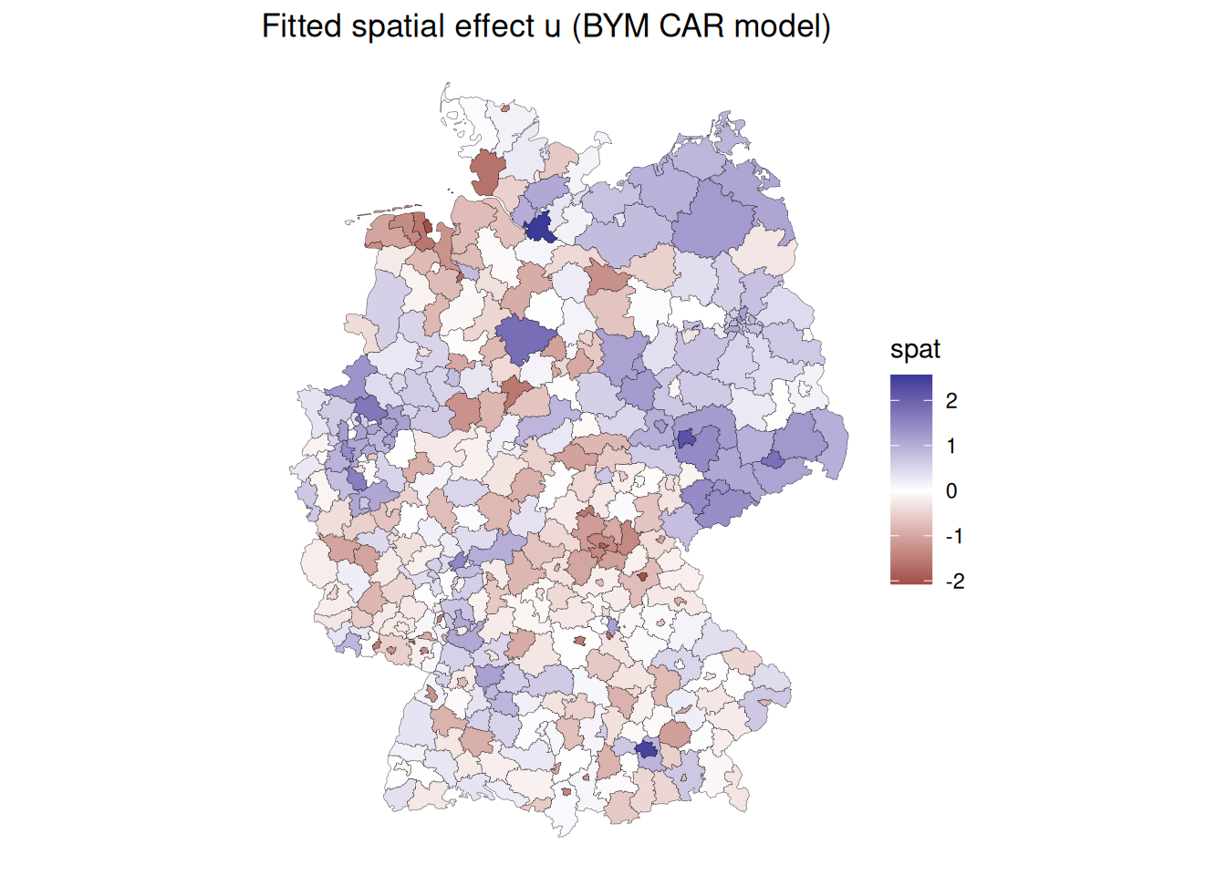
The structured spatial effect \(u_i\) (the CAR part) can be mapped. The summary.random object contains the posterior mean of \(u\) for each region:
# fitted structured spatial effect per regionlk$spat = fit$summary.random$id[seq_len(nrow(lk)), "mean"]library(ggplot2)ggplot(lk) +geom_sf(aes(fill = spat), linewidth =0.1) +scale_fill_gradient2() +theme_void() +labs(title ="Fitted spatial effect u (BYM CAR model)")
NoteExercise
Why is the precision matrix \(Q = D - W\) sparse, and how does that make the CAR model cheap to compute compared to a model with a dense covariance matrix \(\Sigma\)?
Besag, Julian, Jeremy York, and Annie Mollié. 1991. “Bayesian Image Restoration, with Two Applications in Spatial Statistics.”Annals of the Institute of Statistical Mathematics 43 (1): 1–20.
Rue, Havard, and Leonhard Held. 2005. Gaussian Markov Random Fields: Theory and Applications. Chapman; Hall/CRC.