In \(y=X\beta+e\), we call \(\beta\) (or \(X\beta\)) the fixed effects: these are not random. Although \(e\) is a random variable, it does not affect the prediction of \(y\) (only its prediction variance, when predicting a single outcome). As opposed to fixed effects models, random effects models contain (apart from a fixed intercept) only random effects. An example would be \(y = \beta_0 + e\) with \(e \sim \mathcal{N}(0,\Sigma)\) where \(\Sigma\) describes the covariance structure (and hence correlation) of \(e\), and predicting \(y\) involves prediction of \(e\) using similar (for instance nearby in space or time) observations.
Mixed models are models that contain both fixed (beyond intercept) and random effects, an example could be \[y_{ij}=X\beta + u_j + e_{ij}\] where \(y_{ij}\) would be test results of pupil \(i\) in school \(j\), \(e_{ij} \sim \mathcal{N}(0,\sigma^2 I)\) is a random independent residual, and \(u_j\) is the (random) effect of school \(j\) (which has mean zero and variance \(\sigma^2_u\)). Predicting the value for a new student of a observed school \(j\) would involve predicting \(u_j\), but predicting the value for a student from a new (unobserved) school would predict \(u_j\) as zero, but add the variance \(\sigma^2_u\) to the prediction error.
This example reflects possibly the simplest mixed model, that of grouped data: observations belong to a group, and an observation \(y_{ij}\) belonging to group \(j\)
has a variability \(\sigma^2\)within the group (among members of the same group)
has a variability \(\sigma^2 + \sigma_u^2\) overall (among members across groups)
which implies that the correlation of two observations is \(\sigma_u^2/(\sigma^2+\sigma_u^2)\) when they belong to the same group, or zero if they belong to different groups. This leads to a block-diagional covariance (or correlation) matrix.
If there is no group effect, \(\sigma^2_u\) is zero and observations are uncorrelated even if in the same group. It thus is of interest to test whether \(\sigma^2_u\) is significantly larger than zero.
Special cases include
Hierarchical (nested) data: within groups, further grouping takes place, e.g. districts, schools-within-districts, class-within-school.
Longitudinal data: repeated observations are made on the same subjects (e.g. health records on a set of patients repeated over time); the subject (person) is here the grouping factor.
With our Covid data we have time series (repeated observations) over a number of spatial units, and can see this as a longitudinal dataset.
Rows: 1009827 Columns: 7
── Column specification ────────────────────────────────────────────────────────
Delimiter: ","
chr  (1): Landkreis_id
dbl  (5): Bevoelkerung, Faelle_gesamt, Faelle_neu, Faelle_7-Tage, Inzidenz_7...
date (1): Meldedatum

ℹ Use `spec()` to retrieve the full column specification for this data.
ℹ Specify the column types or set `show_col_types = FALSE` to quiet this message.
c19.MS = c19 |>filter(Landkreis_id =="05515")c19.MS.w = c19.MS |>mutate(d =as.numeric(Meldedatum), # day, as numberd_s =scale(d), # scaled to mean 0 sd 1d_rad =2* pi * d /365.25) |># day, yearday -> [0,2*pi]filter(d %%7==0)m =glm(round(cases)~d_s+I(d_s^2)+sin(d_rad)+cos(d_rad), c19.MS.w, family ="poisson")
We can select the Landkreise within 30 km from Stadt Muenster:
library(sf)
Linking to GEOS 3.12.2, GDAL 3.11.4, PROJ 9.4.1; sf_use_s2() is TRUE
c19.MS30km.w = c19.MS30km |>mutate(d =as.numeric(Meldedatum)) |># day, as numbermutate(d_s =scale(d),d_rad =2* pi * d /365.25) |># day, yearday -> [0,2*pi]filter(d %%7==0)
library(lme4)
Loading required package: Matrix
me =glmer(round(cases)~d_s +I(d_s^2)+sin(d_rad)+cos(d_rad)+(1|Landkreis_id), c19.MS30km.w, family ="poisson",control =glmerControl(autoscale =TRUE))
Warning in checkConv(attr(opt, "derivs"), opt$par, ctrl = control$checkConv, : Model is nearly unidentifiable: very large eigenvalue
 - Rescale variables?
summary(me)
Generalized linear mixed model fit by maximum likelihood (Laplace
  Approximation) [glmerMod]
 Family: poisson  ( log )
Formula: round(cases) ~ d_s + I(d_s^2) + sin(d_rad) + cos(d_rad) + (1 |
    Landkreis_id)
   Data: c19.MS30km.w
Control: glmerControl(autoscale = TRUE)

      AIC       BIC    logLik -2*log(L)  df.resid
 10232290  10232333  -5116139  10232278      9471

Scaled residuals:
   Min     1Q Median     3Q    Max
  -110     -9      1     61 400013

Random effects:
 Groups       Name        Variance Std.Dev.
 Landkreis_id (Intercept) 0.6551   0.8094
Number of obs: 9477, groups:  Landkreis_id, 27

Fixed effects:
              Estimate Std. Error  z value Pr(>|z|)
(Intercept)  6.8234086  0.1434081    47.58   <2e-16 ***
d_s         -5.9463236  0.0023321 -2549.82   <2e-16 ***
I(d_s^2)    -5.3338147  0.0019555 -2727.56   <2e-16 ***
sin(d_rad)   0.4982106  0.0003895  1279.21   <2e-16 ***
cos(d_rad)   0.2857715  0.0003815   748.99   <2e-16 ***
---
Signif. codes:  0 '***' 0.001 '**' 0.01 '*' 0.05 '.' 0.1 ' ' 1
optimizer (Nelder_Mead) convergence code: 0 (OK)
Model is nearly unidentifiable: very large eigenvalue
 - Rescale variables?
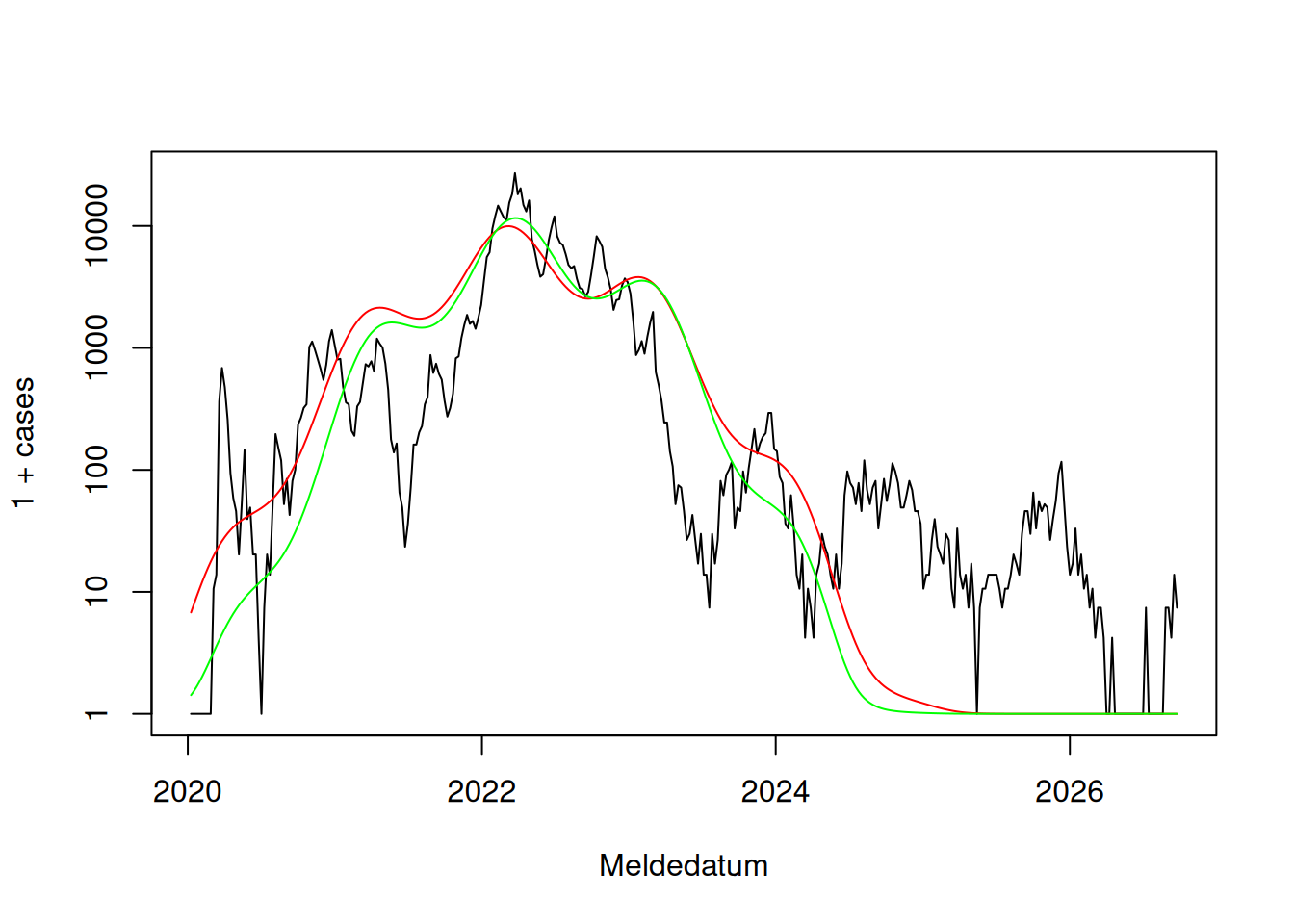
Compare the fits of glm() and glmer():
plot(1+cases ~ Meldedatum,c19.MS.w, type ='l', log ="y")lines(c19.MS.w$Meldedatum, 1+exp(predict(me, c19.MS.w)), col ='red')lines(c19.MS.w$Meldedatum, 1+exp(predict(m)), col ='green')