3  Time series: decomposition, exponential smoothing

This section is based on the Chapter 3 (“Time series decomposition”) and Chapter 8 (“Exponential smoothing”) of Forecasting: Principles and Practice (FPP). The specific sections from these chapters are 3.2–3.4 and 3.6 (components, moving averages, classical decomposition, STL) and 8.1–8.4 (simple exponential smoothing, trend, seasonality, taxonomy).

3.1 Time series decompositions

A common decomposition separates the observations into

  • a trend \(T_t\): a slow, gradual change
  • a periodic effect \(S_t\): a recurrent, cyclic effect with a given frequency (the seasonal component)
  • the remainder \(R_t\): the difference of observations and (trend + periodic)

so that, for an additive decomposition, \[y_t = T_t + S_t + R_t.\]

  • A multiplicative decomposition, \(y_t = T_t \times S_t \times R_t\), fits better when the seasonal swings grow with the level of the series.
  • Taking logarithms turns it into an additive one: \(\log y_t = \log T_t + \log S_t + \log R_t\).

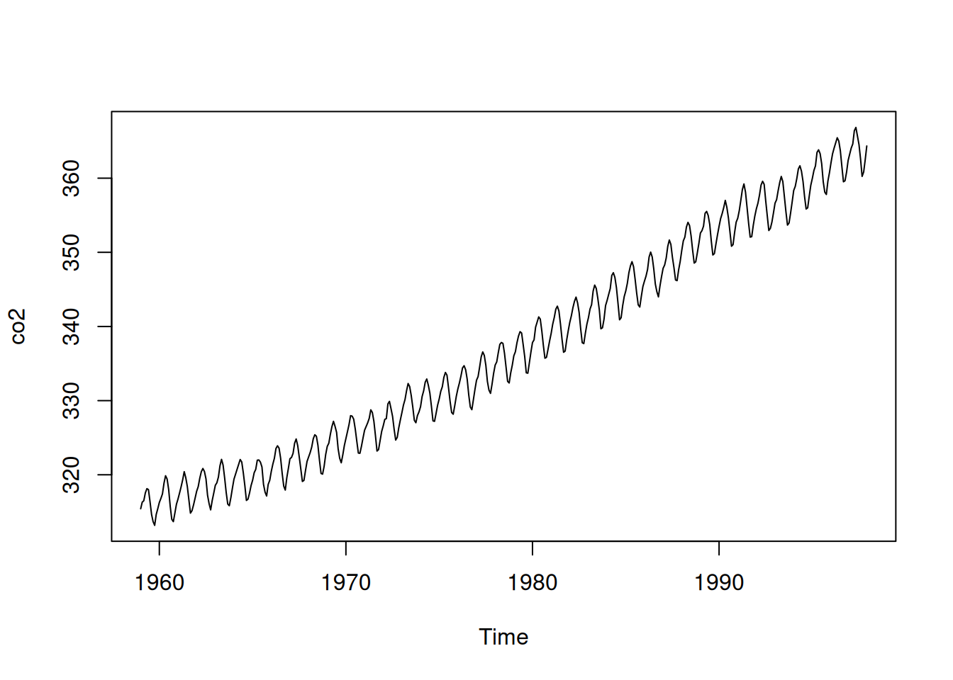
As an example we use the monthly atmospheric CO\(_2\) concentration (ppm) measured at Mauna Loa, 1959–1997:

plot(co2)

The object co2 is of class ts, and provides its frequency (12), the third value of the time series parameters attribute:

attributes(co2)
$tsp
[1] 1959.000 1997.917   12.000

$class
[1] "ts"
  • tsp holds the start (1959.0 is January 1959), the end (1997.917 is December 1997) and the frequency (12 observations per year).
  • The frequency is the length of the seasonal period, \(m\) in FPP. The decomposition functions read it from here, so the series must be a ts object with the right frequency.

3.1.1 Classical decomposition

Classical decomposition (FPP section 3.4) has three steps:

  1. Trend: a centred moving average over one full period. For monthly data this is the “2×12-MA”: the average over 13 months, with half weight for the two outer months. Every calendar month is represented equally, so the seasonal effect averages out.
  2. Seasonal: subtract the trend and average the detrended values per month (all Januaries, all Februaries, …). The 12 averages are shifted to sum to zero and used in every year.
  3. Remainder: \(R_t = y_t - T_t - S_t\).
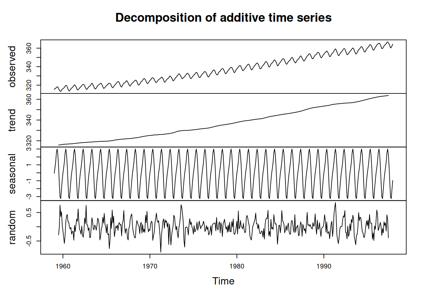
co2_dec <- decompose(co2)
plot(co2_dec)
Known weaknesses:

head(co2_dec$trend, 12)
          Jan      Feb      Mar      Apr      May      Jun      Jul      Aug
1959       NA       NA       NA       NA       NA       NA 315.8613 315.9175
          Sep      Oct      Nov      Dec
1959 315.9767 316.0696 316.1967 316.3287
  • the trend (and hence the remainder) is missing for the first and last six months, because a centred 13-month window does not fit there;
  • the seasonal pattern is identical in every year (co2_dec$figure holds the 12 values);
  • a single unusual value affects both the trend and the seasonal estimate;
  • moving averages flatten sharp rises and falls in the trend.

3.1.2 stl: Seasonal and Trend decomposition using Loess

stl addresses all four weaknesses. Its simplest form is:

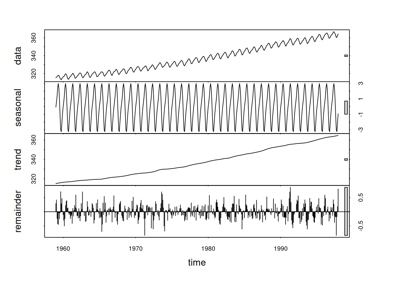
co2_stl <- stl(co2, s.window = "periodic")
plot(co2_stl)
3.1.2.1 Loess in a nutshell

Loess (“locally estimated scatterplot smoothing”) fits a smooth curve through a cloud of points. The smoothed value at a point \(x_0\) is found by:

  1. taking the observations in a window around \(x_0\) (argument span in loess(): the fraction of the data used);
  2. weighting them by their distance to \(x_0\), with zero weight outside the window;
  3. fitting a straight line or a parabola to them by weighted least squares;
  4. taking the value of that fit at \(x_0\).
  • Repeating this for every \(x_0\) gives a smooth curve made of local regressions, without a global formula.
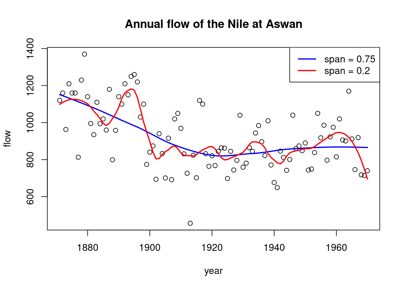
  • The window size controls smoothness: a small window follows the data closely, a large window gives a smooth curve.
nile <- data.frame(year = as.numeric(time(Nile)), flow = as.numeric(Nile))
plot(flow ~ year, nile, main = "Annual flow of the Nile at Aswan")
lines(nile$year, fitted(loess(flow ~ year, nile, span = 0.75)), col = "blue", lwd = 2)
lines(nile$year, fitted(loess(flow ~ year, nile, span = 0.2)), col = "red", lwd = 2)
legend("topright", c("span = 0.75", "span = 0.2"), col = c("blue", "red"), lwd = 2)
Compared to classical decomposition, STL

  • gives estimates up to both ends of the series,
  • lets the seasonal pattern change over time, at a rate set by s.window,
  • lets the user control the smoothness of the trend with t.window,
  • can be made robust to outliers (robust = TRUE),
  • works for any seasonal period, not only months or quarters.

Its limitations:

  • it only does additive decompositions (log-transform the series first for multiplicative behaviour);
  • the windows have to be chosen by the user;
  • it describes the past rather than forecasting the future.

The components are stored as a multivariate time series in the element time.series of the stl object:

co2_per <- stl(co2, s.window = "periodic")
head(co2_per$time.series)
            seasonal    trend   remainder
Jan 1959 -0.06100103 315.1954  0.28564410
Feb 1959  0.59463870 315.3023  0.41305456
Mar 1959  1.32899651 315.4093 -0.23825306
Apr 1959  2.46904706 315.5147 -0.42371128
May 1959  2.95704630 315.6201 -0.44711820
Jun 1959  2.31835208 315.7194 -0.03777682
  • The seasonal component is co2_per$time.series[, "seasonal"].
  • acf() applied to a monthly ts labels the lags in years: lag 1.0 means 12 months.
NoteExercise

Look at autocorrelation plots of the seasonal, trend, and remainder components of the stl() plot above, describe what you see, and explain why it is like that.

NoteExercise

Decrease the smoothness of the trend component and describe how this affects the seasonal and remainder components. (Use the argument t.window, with an odd value smaller than the default of 19.)

3.2 Exponential smoothing

3.2.1 Two simple benchmarks

To predict a new observation \(y_{T+1}\) from a time series \(y_1, \ldots, y_T\):

  • The naïve forecast uses the last observed value: \[\hat{y}_{T+1|T} = y_T\] It ignores everything before \(y_T\). This is basically predicting tomorrow’s weather from that of today, and is often used as a benchmark for its simplicity (and, in case of weather, performance).
  • If all past observations are equally (un)informative, it makes sense to use their mean: \[\hat{y}_{T+1|T} = \frac{1}{T}\sum_{t=1}^T y_t\]
  • The notation \(\hat{y}_{T+1|T}\) reads “the forecast for time \(T+1\), given the observations up to time \(T\)”.
  • Both are weighted averages of past observations: the naïve forecast gives weight 1 to \(y_T\) and 0 to all others, the mean gives weight \(1/T\) to each.

3.2.2 Simple exponential smoothing (SES)

3.2.2.1 Weighted average form

A compromise between these two extremes is exponential smoothing, a weighted average with weights that decay exponentially as observations get older:

\[\hat{y}_{T+1|T} = \alpha y_T + \alpha(1-\alpha) y_{T-1} + \alpha(1-\alpha)^2 y_{T-2} + \cdots = \sum_{j=0}^{T-1} \alpha(1-\alpha)^j\, y_{T-j} \;+\; (1-\alpha)^T \ell_0\]

with \(0 \le \alpha \le 1\).

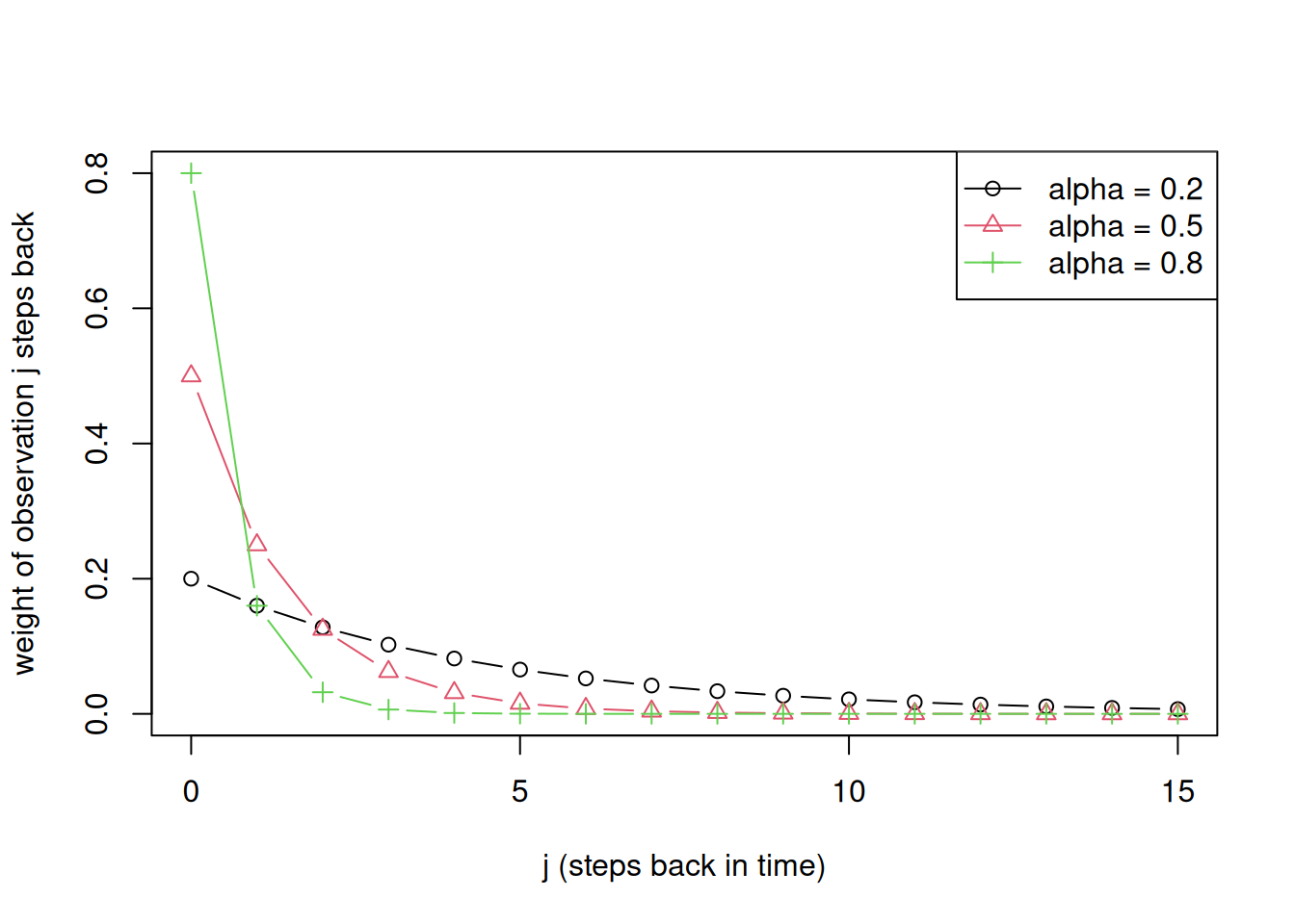
  • The observation \(j\) steps back, \(y_{T-j}\), gets weight \(\alpha(1-\alpha)^j\).
  • For \(\alpha\) close to 1, nearly all weight goes to the last observation: the naïve forecast.
  • For small \(\alpha\), the weights decay slowly and many past observations contribute. For \(\alpha = 0\) the forecast is the constant \(\ell_0\); if \(\ell_0\) is chosen to fit the data best, that constant is the mean.
  • The weights for \(j = 0, \ldots, T-1\) add up to \(1 - (1-\alpha)^T\). The remaining weight \((1-\alpha)^T\) goes to \(\ell_0\), an initial value representing the level before the first observation.
j <- 0:15
alphas <- c(0.2, 0.5, 0.8)
w <- sapply(alphas, function(a) a * (1 - a)^j)
matplot(j, w, type = "b", pch = 1:3, lty = 1, col = 1:3,
        xlab = "j (steps back in time)", ylab = "weight of observation j steps back")
legend("topright", legend = paste("alpha =", alphas), pch = 1:3, col = 1:3, lty = 1)
3.2.2.2 Component form: the level

The same method can be written as a recursion. The level \(\ell_t\) is the estimate of the underlying value of the series at time \(t\), with the noise smoothed out:

\[ \begin{aligned} \text{forecast equation:} \quad & \hat{y}_{t+h|t} = \ell_t \\ \text{level equation:} \quad & \ell_t = \alpha\, y_t + (1-\alpha)\, \ell_{t-1} \end{aligned} \]

  • The new level is a weighted average of the new observation and the previous level. Substituting the level equation into itself repeatedly gives back the weighted average form.
  • The forecast for every future time step is the last level \(\ell_T\): SES forecasts are flat.
  • The component form is easier to extend: trend and seasonal components each get their own equation.

3.2.3 Holt’s linear trend method

SES works well for data with a constant or slowly wandering mean, without trend or seasonal component. For data with a trend, Holt’s method adds a second component, the slope \(b_t\):

  • FPP and R’s HoltWinters call \(b_t\) the “trend”, but it is the slope of the local trend line: the expected change per time step. (In a decomposition, the trend \(T_t\) is the whole smooth curve.)
  • The trend is now described by two numbers: the level \(\ell_t\) (where the series is now) and the slope \(b_t\) (how fast it is moving).
  • Forecasts follow a straight line from the current level with the current slope:

\[ \begin{aligned} \text{forecast:} \quad & \hat{y}_{t+h|t} = \ell_t + h\, b_t \\ \text{level:} \quad & \ell_t = \alpha\, y_t + (1-\alpha)(\ell_{t-1} + b_{t-1}) \\ \text{slope:} \quad & b_t = \beta^*(\ell_t - \ell_{t-1}) + (1-\beta^*)\, b_{t-1} \end{aligned} \]

  • Level: as in SES, but the previous estimate is now where we expected to be: the previous level plus one step of slope, \(\ell_{t-1} + b_{t-1}\) (the one-step forecast).
  • Slope: \(\ell_t - \ell_{t-1}\), how much the level just moved, is a new but noisy measurement of the slope. It is averaged with the previous slope using \(\beta^*\); a small \(\beta^*\) means the slope changes slowly.

As an example we take the seasonally adjusted CO\(_2\) series, with the seasonal component of the stl result above removed. HoltWinters with gamma = FALSE fits Holt’s method:

co2_sa <- co2 - co2_stl$time.series[, "seasonal"]   # seasonally adjusted
holt <- HoltWinters(co2_sa, gamma = FALSE)
c(alpha = holt$alpha[[1]], beta = holt$beta[[1]])
     alpha       beta 
0.77943817 0.02762752 
holt$coefficients    # final level (a) and slope (b, in ppm per month)
         a          b 
365.103833   0.140949 
plot(fitted(holt))
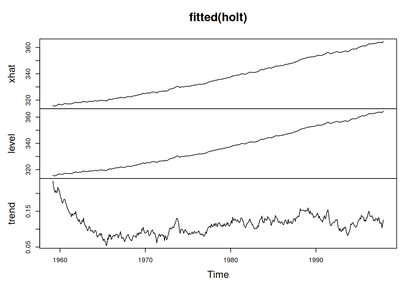
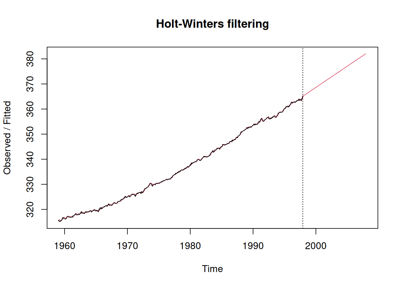
The panels show the one-step forecasts (xhat), the level and the slope (named trend in R). Forecasting ten years ahead:

plot(holt, predict(holt, n.ahead = 120))
3.2.4 Holt-Winters: adding seasonality

See section 8.3 in the FPP book.

  • Holt-Winters adds a third component: a set of \(m\) seasonal indices, one per season (12 for monthly data).
  • An index says how far above or below the level that season typically is, for instance “March is usually 1.3 ppm above the level”.
  • \(s_{t-m}\) is the index of the same season one period (year) earlier: the most recent estimate for that season.

For the additive method:

\[ \begin{aligned} \text{forecast:} \quad & \hat{y}_{t+h|t} = \ell_t + h\, b_t + s_{t+h-m(k+1)} \\ \text{level:} \quad & \ell_t = \alpha\,(y_t - s_{t-m}) + (1-\alpha)(\ell_{t-1} + b_{t-1}) \\ \text{slope:} \quad & b_t = \beta^*(\ell_t - \ell_{t-1}) + (1-\beta^*)\, b_{t-1} \\ \text{season:} \quad & s_t = \gamma\,(y_t - \ell_{t-1} - b_{t-1}) + (1-\gamma)\, s_{t-m} \end{aligned} \]

  • Level: the new observation is first seasonally adjusted, \(y_t - s_{t-m}\), so that a regular seasonal peak is not mistaken for a jump in the level.
  • Slope: as in Holt’s method.
  • Season: \(y_t - (\ell_{t-1} + b_{t-1})\), how far the new observation lies above the expected non-seasonal value, is a new measurement of this season’s effect. It is averaged with the previous index of the same season.
  • Forecast: the subscript \(t+h-m(k+1)\), with \(k\) the integer part of \((h-1)/m\), only makes sure that the most recent index of the forecasted season is used.

How the seasonal indices behave:

  • Each index is updated only once per period: the March index only changes when a March observation arrives. Holt-Winters effectively runs \(m\) small exponential smoothers side by side, each seeing one observation per year.
  • This is the one-sided counterpart of smoothing the cycle-subseries in stl.
  • \(\gamma\) plays a role similar to s.window: \(\gamma\) close to 0 keeps the seasonal pattern nearly constant (like "periodic"), a larger \(\gamma\) lets it change faster.

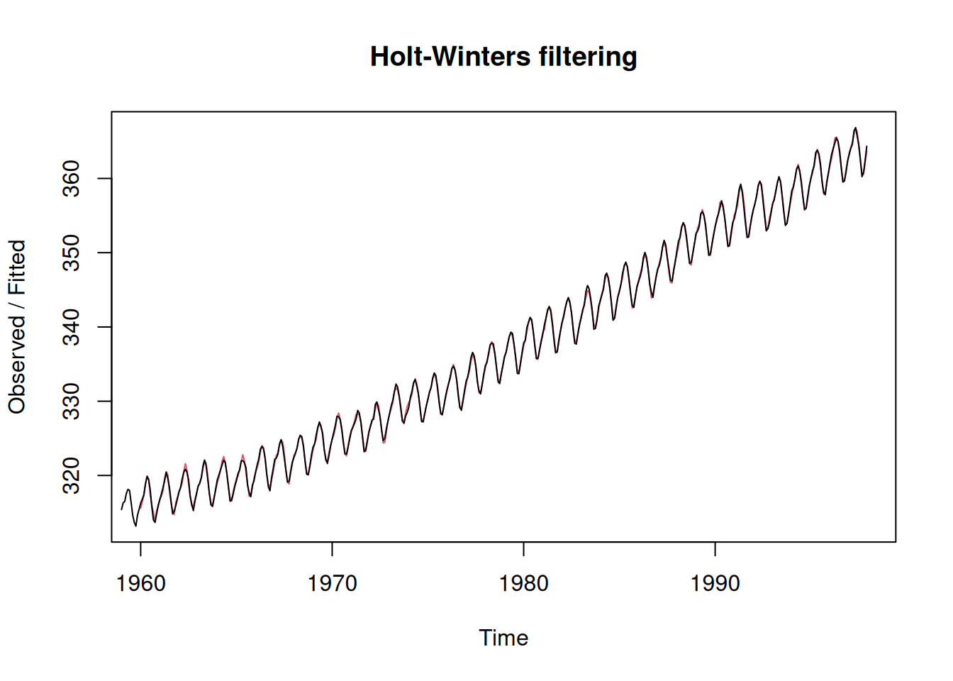
HoltWinters(co2) fits the additive method, estimating \(\alpha\), \(\beta\) and \(\gamma\) by minimising the sum of squared one-step forecast errors with optim:

hw <- HoltWinters(co2)
c(alpha = hw$alpha[[1]], beta = hw$beta[[1]], gamma = hw$gamma[[1]])
      alpha        beta       gamma 
0.512648444 0.009497669 0.472886788 
plot(hw)
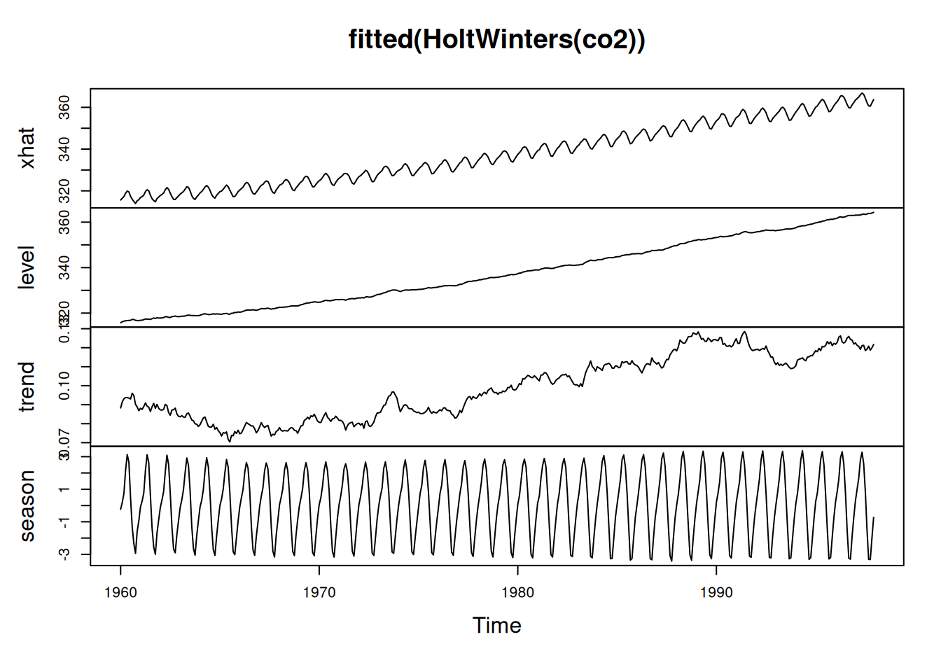
The fitted components over time:

plot(fitted(HoltWinters(co2)))
NoteExercise

In this plot, what is different from the decomposition obtained by stl()?

Look at the names of the panels and what they contain, at the time range of the plot, and at which observations each component at time \(t\) is based on.

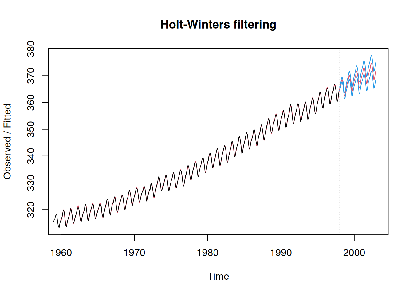
Forecasting five years ahead, with prediction intervals:

plot(hw, predict(hw, n.ahead = 60, prediction.interval = TRUE))
3.3 Note

This content is created using AI model (claude Opus 5)